


In order to study the relationship between life-history ecology and morphology, we must first find ways to accurately quantify the shape of our newts and their bones. To do this, we primarily use two complementary approaches: linear measurements and 3D geometric morphometry.
Measuring the Body: Linear Measurements
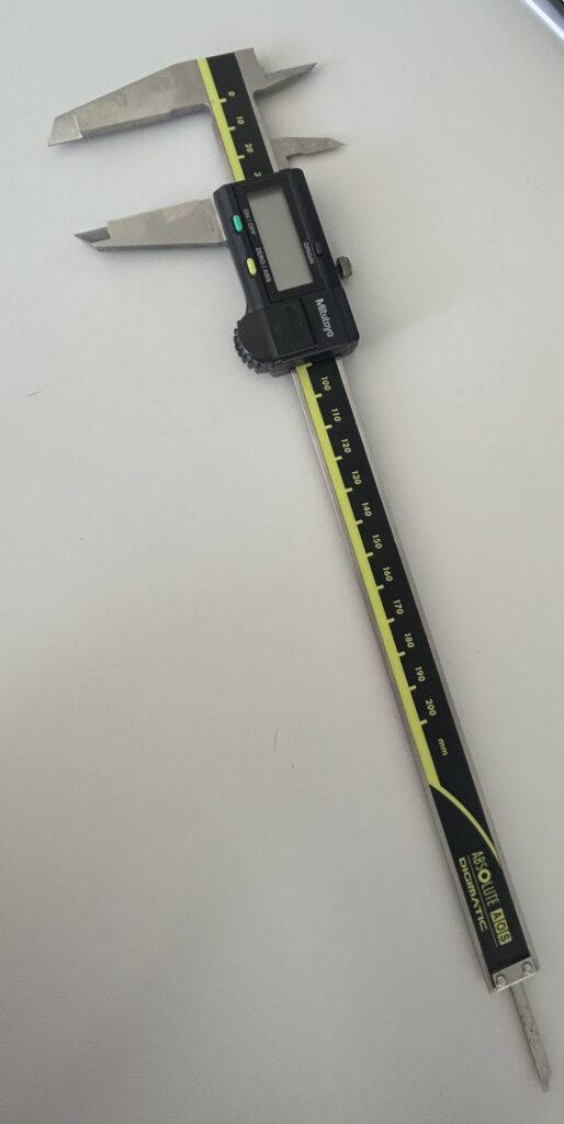
Linear measurements are simple distance measurements taken using a precision instrument, such as a caliper.
It allow us to measure the overall size of newts, as well as different parts of their bodies, such as the length of their legs or toes.
These measurements thus allow us to convert each animal’s morphology into numerical data, which we can then compare across individuals and populations. In particular, they enable us to determine whether certain body parts are proportionally larger or smaller depending on the life cycle of the newts.
Studying Bones in 3D: Geometric Morphometry
To study the shape of bones, particularly those of the skull, in greater detail, we use a method called 3D geometric morphometry.
The specimens are first scanned using X-rays, which allows us to reconstruct their bones as three-dimensional digital models.
To learn more about how we scan them, click here!
We then place anatomical landmarks, on these 3D models. These points are positioned on specific, easily identifiable anatomical structures, for example, at the end of a bone, where two structures meet, or on a distinctive anatomical feature. The same landmarks are used for all individuals in a given analysis, allowing for reproducible comparisons of their shapes.
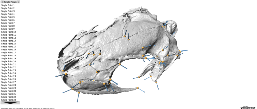
There are different types of landmarks. Type 1 landmarks generally correspond to points where multiple anatomical structures meet, while Type 2 landmarks correspond to points defined by a geometric characteristic, such as a curve or an end point. Type 3 landmarks, on the other hand, are defined primarily by their position relative to other structures, for example, the point farthest from or closest to another part of the bone.
Once we have obtained the 3D coordinates of these landmarks, we use a Procrustes superimposition to align the specimens. This process removes differences in position, orientation, and overall size, allowing us to focus specifically on differences in shape.
We can then compare bone shapes across individuals and populations.
What should we do with this data?
We can then visualise this data using principal component analysis (PCA). This allows us to summarise a large number of morphological variables into a few axes that represent the main sources of variation between individuals.
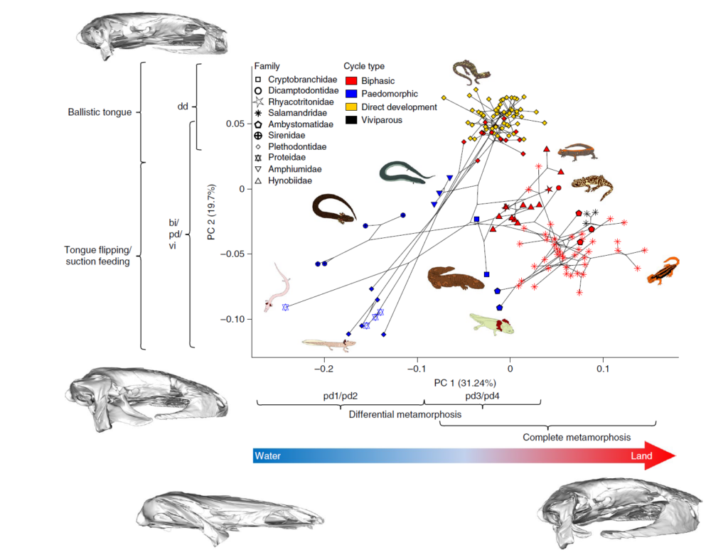
On the graph, each point represents an individual. The first two axes, PC1 and PC2, correspond to the main directions of variation: individuals close to one another have similar morphology, whereas those further apart exhibit greater differences in shape. This makes it possible, in particular, to see whether certain groups, such as different life cycle types, tend to differ morphologically.
But these are simply observations, and more advanced statistical analyses can then be applied.